Tutorial
Fs Peptide
The command-line tool is
msmb. Check that it’s installed correctly and read the help options:msmb -h
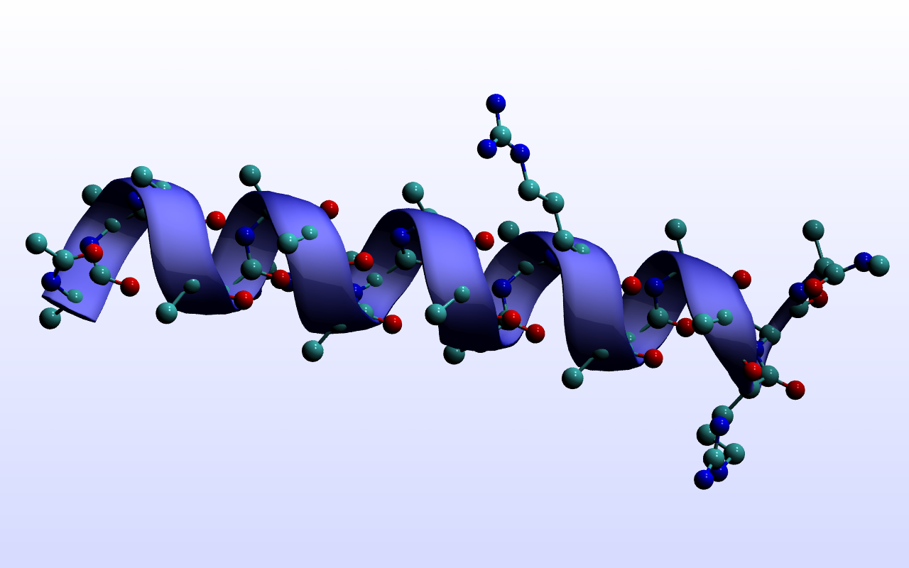
In your own research, you probably have a large molecular dynamics dataset that you wish to analyze. For this tutorial, we will perform a quick analysis on a simple system: the Fs peptide.
We’ll use MSMBuilder to create a set of sample python scripts to sketch out our project:
msmb TemplateProject -h # read the possible options
msmb TemplateProject
This will generate a hierarchy of small scripts that will handle the boilerplate and organization inherent in MSM analysis.:
.
├── analysis
│   ├── dihedrals
│   │   ├── tica
│   │   │   ├── cluster
│   │   │   │   ├── msm
│   │   │   │   │   ├── timescales.py
│   │   │   │   │   ├── timescales-plot.py
│   │   │   │   │   ├── microstate.py
│   │   │   │   │   ├── microstate-plot.py
│   │   │   │   │   ├── microstate-traj.py
│   │   │   │   ├── cluster.py
│   │   │   │   ├── cluster-plot.py
│   │   │   │   ├── sample-clusters.py
│   │   │   │   ├── sample-clusters-plot.py
│   │   │   ├── ftrajs -> ../ftrajs
│   │   │   ├── tica.py
│   │   │   ├── tica-plot.py
│   │   │   ├── tica-sample-coordinate.py
│   │   │   ├── tica-sample-coordinate-plot.py
│   │   ├── featurize.py
│   │   ├── featurize-plot.py
│   ├── gather-metadata.py
│   ├── gather-metadata-plot.py
├── 0-test-install.py
├── 1-get-example-data.py
└── README.md
Each subsequent step in the MSM construction pipeline is a subdirectory.
Retrieve the Fs peptide example data by running:
python 1-get-example-data.py
Ensure that you now have a directory named
fs_peptidewith 28xtctrajectories in it and apdbtopology file namedfs-peptide.pdb. Feel free to load one of these trajectories in VMD to get a sense of what they look like. Ensure that the symlinkstop.pdbandtrajsresolve to the correct place. We use symlinks to map your filenames to into “standard” msmbuilder names. For example, if your set of trajectories was stored on another partition, you could use a symlink to point to the folder, name ittrajs, and the scripts will work without modification.Begin our analysis:
cd analysis/We first generate a list of our trajectories and associated metadata. Examine the
gather-metadata.pyscript. Note that it uses thextcfilenames to generate an integer key for each trajectory. The script also extracts the length of each trajectory and stores the xtc filename:python gather-metadata.py python gather-metadata-plot.py
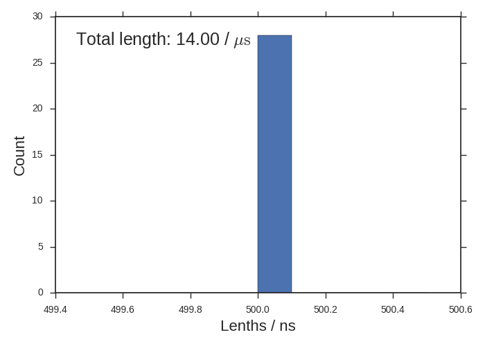
Sometimes you’ll have many different length-ed trajectories and this histogram will be interesting. All of our trajectories are 500 ns though.
The plot script contains several example functions of computing statistics on your dataset including aggregate length. It will also generate an
htmlrendering of the table of metadata. Exercise: modify the script to genereatepngimages intead ofpdfvector graphics for the plots. Editor’s note: usepdffor preperation of manuscripts because you can infinitely resize your plots.We’ll start reducing the dimensionality of our dataset by transforming the raw Cartesian coordinates into biophysical “features”. We’ll use dihedral angles. The templated project also includes subfolders
landmarksandrmsdfor alternative approaches, but we’ll ignore those for now:cd dihedrals/Examine the
featurize.pyscript. Note that it loops through our trajectories using the convenience functionitertrajs(which only ever holds one trajectory in RAM) and callsDihedralFeaturizer.partial_transform()on each. Read more about featurizers and MSMBuilder API patterns. Run the scripts:python featurize.py python featurize-plot.py
The plots will show you a box and whisker plot of each feature value. This is not very useful, but we wanted to make sure you can plot something for each step. Exercise: include chi1 and chi2 angles in addition to the default phi and psi angles.
Dihedrals are too numerous to be interpretable. We can use tica to learn a small number of “kinetic coordinates” from our data:
cd tica/Examine
tica.py. Note that it loads the feature trajectories, learns a model from them by callingfit()and then transforms the feature trajectories into “tica trajectories” by callingpartial_transform()on each (see api patterns). The MSMBuilder API does not keep track of units. Our data was saved every 50 ps (Editor’s note: this is way too frequent for a “real” simulation). The template script for learning our tica model sets thelag_timeparameter to10. This means 10 steps in our data. This translates to 500 ps here. Let’s use something a little longer like 5 ns (= 100 steps). Edit thelag_timeparameter to 100 and learn the model:vim tica.py # edit lag_time -> 100 python tica.py python tica-plot.py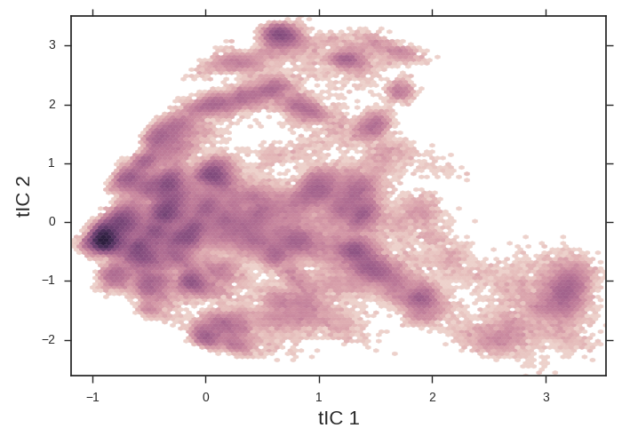
tICA heatmaps provide a convenient 2d projection of your data onto which you can overlay more interesting info.
The tICA plotting script makes a 2d histogram of our data. Note the apparent free energy well on the left of the figure. We might suspect that this is the folded state and the x-axis is an unfolding coordinate. We’ll use this tica heatmap as a background for our further plots. tICA is extremely useful at taking hundreds of dihedral angles (for example) and distilling it into a handful of coordinates that we can plot.
We can sample configurations along a tIC to inspect what that tIC “means”. Another common strategy for interpreting tICs is to inspect prominent (most non-zero) coefficients corresponding to particular features (dihedrals). A common tactic is to color residues based on their tIC loading. Example scripts to set up VMD for this will be included in a later release. Here, we simply draw configurations along a tIC direction:
python tica-sample-coordinate.py
python tica-sample-coordinate-plot.py
The first tIC is roughly a folding coordinate.
This produces a trajectory of conformations, saved as
tica-dimension-0.xtc. Exercise: Save the conformations as adcdtrajectory instead. You can load this trajectory in VMD and inspect the particular tIC:vmd top.pdb tica-dimension-0.xtc
Align the structures and apply some “smoothing”. Exercise: Sample the second tIC. Note that it probably isn’t an interesting coordinate in this case.
We can group conformations that interconvert rapidly by using off-the-shelf clustering algorithms on our kinetic coordinates (tICs):
cd cluster/By default, we generate 500 clusters using a form of KMeans. Read more about clustering. Exercise: try a different number of clusters or a different clustering algorithm. Run the clustering scripts:
python cluster.py
python cluster-plot.py
Note that the tIC heatmap provides a convenient space onto which we project our cluster centers.
With our states defined, we count the transitions between them. An MSM is simply states and rates. First we make a “microstate” MSM consisting of many, small states:
cd msm/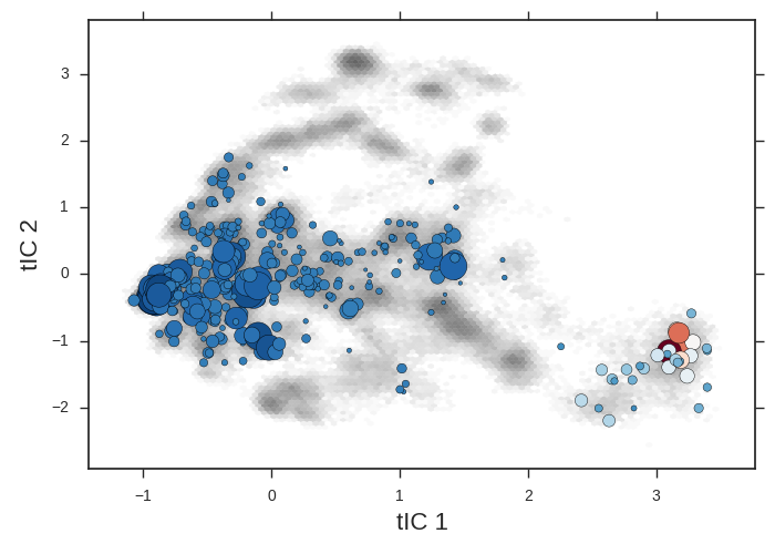
The microstate centers are shown as circles on the tIC heatmap. They are sized according to state population. They are colored according to the first dynamical eigenvector. The slowest processes is a transition from red states to blue.
The MSM lag-time is a parameter that cannot be optimized using gmrq. You can use the
timescales.pyscript to check how the model timescales would react to changing the lag-time. We’ll just use a lag-time of 5 ns. Remember from above that we have to keep track of units. 5 ns is 100 steps. Editmicrostate.pyand setlag_time = 100:vim microstate.py # edit lag_time python microstate.py python microstate-plot.pyGenerate a sample trajectory from the MSM:
python microstate-traj.py
By default, each frame will be 1 lag-time unit. Here, that is 5 ns. Exercise: Use the
n_stepsandstrideparameter to sample a 200 frame movie with 50 ns steps. You can load the trajectory in VMD and watch the Fs-peptide stochastically fold and unfold:vmd top.pdb msm-traj.xtc